
|
 |
|
A Magical Trick by Brian Beckman PhD
The Magic Formulae (Physics of Racing The Magic Formula:
Longitudinal Version, The Magic Formula:
Lateral Version, Combination Slip,
Combination Grip) for grip versus slip have some disadvantages
for the simulation programmer. Chief among them are the complicated mathematical structure and the large number of parameters. In this instalment, we
show a much simpler mathematical expression that mimics the most important, overall features of the Magic Formulae with many fewer
parameters. This "Magic Trick" formula is much easier to code and debug, requires much less computing horsepower, and differs by less
than 10% almost everywhere from Pajecka: probably sufficiently accurate for gaming simulation. Just to tantalize you, let me offer
the following two plots:
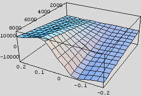 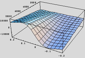 The one on the left is the full, longitudinal Magic Formula. The one on the right is a plot of The full Magic Formulae were developed for professional research in tyre dynamics. That is why they have so many parameters: they must model everything from large truck tyres to off-road tyres to racing slicks, plus every subtlety of behaviour of every different type of tyre. For simulation and gaming, however, the most important behaviour is simply breakaway instability: the decrease in grip with increasing slip beyond the limits. Minor bumps and wiggles in the curves may be critical to capture differences in brand or type or rubber compound, but they are probably overkill even for detailed simulations like Grand Prix Legends or NASCAR 4. Since the Magic Formulae are "the only game in town," however, simulation programmers tend to use them whilst purposefully wasting their subtle capabilities. In fact, my own presentations of the formulae set most of the parameters to zero value, and mine was derived directly from Genta's (Motor Vehicle Dynamics, pub. World Scientific, 1999). So the available modelling 'dynamic range,' as it were, of the Magic Formulae, seems too large for our applications. We need a simpler formula. After playing around for a little while, I found that the following bears an uncanny resemblance to the Magic Formula, but with only three parameters, (A, B, P): This is just a generic form of the formula, in which Fhorizontal could be Flateral or Flongitudinal, and could be slip angle or slip ratio. In other words, the sketch above can account for either the longitudinal or the lateral Magic Formula. Let's analyse the longitudinal formula in detail, using Mathematica (MMA, introduced in Four-Wheel Weight Transfer). I make reference to the longitudinal formula without copying it here, so you will need longitudinal formula on hand to go forward from this point. You will also need familiarity with Mathematica, and possibly to have its manual on hand. Encode the Pajecka b parameters twice as vectors, one symbolic, one as numeric rules for Genta's supposed Ferrari: ClearAll [b]; b[symbolic] = {b0, b1/MN, b2/K, b3/MN, b4/K, b5/KN, b6/KN2, b7/KN, b8, b9/KN, b10}; b[ferrari] = {b01.65, b10., b21688., b30., b4229., b50., b60., b70., b8-10., b90., b100.}; So, it's meaningful to do things like this b[symbolic] /. b[ferrari] Define some helper functions and more numeric rules (the nomenclature will be obvious if you have one eye on the equations in The Magic Formula: Longitudinal Version; this is a straight transcription): b[n_Integer] := b[symbolic] [[n+1]]; muPeak[fz_] := b[1] fz + b[2] bigD[fz_] := muPeak[fz] fz bb0d[fz_] := (b[3] fz2 + b[4] fz) E-b[5]fz bigB[fz_] := numRulez = {MNMegaNewton, KNKiloNewton, K1000, Kilo1000, Mega1000000, 0.0, 1.1, -1.1, 100.100}; In our numerical exposition of the formula in The Magic Formula: Longitudinal Version, we found the constant 0.0822203 popping up over and over. So, test the current forms to see if the same constant appears by substituting the Ferrari's data into them: Simplify[bigB[aa KN] /. b[ferrari]] /. numRulez 0.0822203 Add more helpers: bigS[sigma_, fz_] := (100 sigma) + b[9] fz + b[10] bigE[fz_] := b[6] fz2 + b[7] fz + b[8] and, finally, the whole formula: fx[sigma_, fz_ ] := Module[ {SB = bigS[sigma, fz] bigB[fz], e = bigE[fz], bigD[fz] Sin[b[0] ArcTan[SB + e (ArcTan[SB] - SB)]]] Make a version of the formula with the Ferrari substituted in: fxNum[s_, fz_] := fx[s, fz] / Newton /. b[ferrari] /. numRulez Evaluate this final formula symbolically to check against part 21, then numerically, with a big plot: fxNum[sig, zed] (1.688 zed Sin[ 1.65 ArcTan[8.22203 sig - 10. (-8.22203 sig + ArcTan[8.22203 sig])]]) Plot3D[fxNum[sigma, fz Newton], {sigma, -.20, .20}, {fz, 1, 8000}, ViewPoint{-1.3, 2.4, 1.5}]; 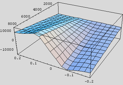 We've successfully reproduced the Magic Formula, and this is the plot we want to emulate. So far, there has been nothing new, just recasting of familiar territory in Mathematica, where we can manipulate the data and formulas. The new function is vastly easier to write down (that's the whole point!), and the plot looks very similar: fx2Num[s_, fzN_, A_, B_, P_ ] := B fzN s / (1 + Abs[A s]^ P) Plot3D[fx2Num[sig, fzn, 9.625, 31, 2.375], {sig, - .20, .20}, {fzn, 1, 8000}, ViewPoint {-1.3, 2.4, 1.5}]; 
It remains only to show how to obtain the parameter values The short answer is by the least squares method. The slightly longer answer is to subtract the two plots, sum up the squares of the differences, and then find those values of (A, B, P) that minimize this sum of squares. In the following, I use the already known best values, as if they were handed to me by an oracle. The reason I do this is that it keeps the presentation short: you don't have to look at a bunch of trial-and-error plots gone haywire. But imagine that you don't know the values as I talk you through the process of finding them. I talk you through it because the process is generic, meaning that you can apply it to parameter-searching problems similar to this one. First, plot the errors, that is, the difference between the two forms. errdiff1[sig_, fzn_, A_, B_, P_] := (fxNum[sig, fzn Newton] - fx2Num[sig, fzn, A, B, P]) Timing[Plot3D[errdiff1[sig, fzn, 9.625, 31, 2.375], {sig, -.20, .20}, {fzn, 1, 8000}, ViewPoint{-1.3, 2.4, 1.5}]] 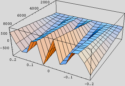 {0.812 second, - SurfaceGraphics -} Note that the maximum magnitude of the errors is about 800 N, or less than 10% of the maximum force. Given that the shape of the plot is very similar to that of Pajecka, hence, that the behavioural characteristics will be similar, we should feel encouraged to go on, with the reservation that the errors are large at the origin, where the force is small. In fact, the errors do reach around 32% at the origin, as shown in the next plots errpct[sig_, fzn_, A_, B_, P_] := 100 Abs[(1 - fx2Num[sig, fzn, A, B, P] / fxNum[sig, fzn Newton])] TimingPlot[Plot3D[errpct[sig, fzn, 9.625, 31, 2.375], {sig, -.20, .20}, {fzn, 1, 8000}, ViewPoint{-1.3, 2.4, 1.5}]] 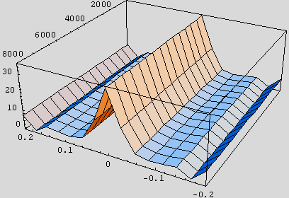
However, this does not concern me very much, for a couple of reasons. First, consider the fact that most authors are satisfied to use a linear approximation near the origin. Witness the ever-present cornering stiffness in the lateral case. Neither of our forms is particularly linear and would probably deviate from a linear approximation at least as much as they deviate from one another. If a linear approximation to Pajecka is good enough, why wouldn't a handy nonlinear approximation, which happens to have much better overall behaviour, be good enough? Secondly, in racing simulation, we are seldom in the linear region, and we should be much more concerned with the differences near the force maxima, around s = 0.15. At these values, the errors are much smaller, well under 10%. Turning attention back to the plot of errors, notice that some errors are negative and some are positive. That's the reason that we square them: we want the overall sum to be positive for any values of the parameters. We don't want to add negative errors to positive errors and risk getting a low estimate of variance. Note that we might just as well add the absolute values rather than the squares, but squares are much easier to manage symbolically since they are smooth (differentiable) at the origin. Also, squaring errors amounts to an assumption of independence: it treats the errors just like components of a vector in a large-dimensional Euclidean space. Historically, a considerable number of tools were developed to solve such problems analytically (symbolically), so squares it is. In fact, we could approach the present problem symbolically with Mathematica, and we might do that in a later instalment. For now, in the interest of getting results quickly, we do a brute-force search for the best values of (A, B, P). I like to call this search method archaeological, because it's the same one archaeologists use to search a site for artefacts: grid off the search space, then exhaustively examine each grid cell. Since (A, B, P) spans a three-dimensional space, each cell is a cube, just like a real archaeological dig! Note that archaeological search is dumb: it's much more clever to do hill climbing (steepest descent), simulated annealing, Kernighan-Lin, or symbolic solution. However, precisely because archaeological search is so dumb, it's nearly trivial to code and debug. For many problems, human coding time is more valuable than computer time, and that's the case here. So we let the computer do a bit of extra heavy sweating to save our effort. Note we don't have to do these searches in real time in the simulation: we only have to do one search for each set of Pajecka parameters. If a simulation has 20 different kinds of tyres, 20 searches are done ahead of time and the (A, B, P) parameters go into the simulation in a table. If it were necessary to search in real time, then cleverer methodology and coding would be justified. First, zoom in on some two-dimensional slices of the search space and see if we're near a minimum. Look at s2[A_, B_, P_] := Module[ {v = 0}, Do[v += errdiff2[s, f, A, B, P], {s, -0.2, 0.2, 0.02}, {f, 1, 8000, 500}]; v] Timing[Plot3D[s2[i, j, 2.375], {i, 8, 12}, {j, 27, 37}, ViewPoint{-1.3, 2.4, 1.5}]] 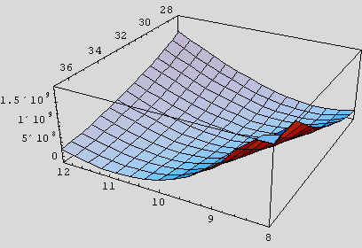
{247.496 Second , - SurfaceGraphics -} Notice the timing: this plot took some time to produce, so we're having to wait a little for results. More importantly, notice the broad trough at the bottom, suggesting that a minimum can be found in the trough somewhere. A contour plot of the same region gives us even more confidence that we're on the correct archaeological site and can begin digging: Timing[ContourPlot[s2[i, j, 2.375], {i, 6, 14}, {j, 17, 47}]] 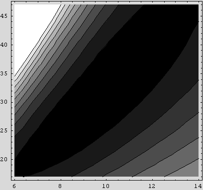
{256.328 Second , - ContourGraphics -} The contour plot shows that the trough is roughly elliptical and most likely holds a minimum of Look at another slice, this time fixing B. Timing[Plot3D[s2[i, 31, k], {i, 9.5, 9.75}, {k, 2.25, 2.5}, ViewPoint{-1.3, 2.4, 1.5}]] 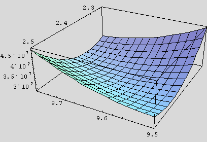
{262.708 Second , - SurfaceGraphics -} Timing[ContourPlot[s2[i, 31, k], {i, 9.5, 9.75}, {k, 2.25, 2.5}]] 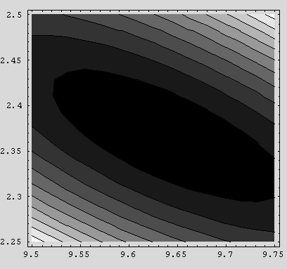 This slice has almost the same character as the previous one: a broad, narrow trough that likely contains the minimum of run[step_, {alo_, ahi_}, {blo_, bhi_}, {plo_, phi_}] := Timing[Module[{ax = 0, bx = 0, px = 0, ebest = $MaxMachineNumber, etest = 0, abest = 0, bbest = 0, pbest = 0}, Do[ etest = s2[ax, bx, px]; If[etest < ebest, ebest = etest; abest = ax; bbest = bx; pbest = px; Print[{ebest, abest, bbest, pbest}], Null], {ax, alo, ahi, step}, {bx, blo, bhi, step}, {px, plo, phi, step}]; {ebest, abest, bbest, pbest}]] run[1 / 8., {9.5, 9.75}, {30.50, 31.50}, {2.250, 2.5}] {4.08339 x 10⁷, 9.5, 30.5, 2.25} {2.90981 x 10⁷, 9.5, 30.5, 2.375} {2.90128 x 10⁷, 9.625, 30.875, 2.375} {2.89942 x 10⁷, 9.625, 31., 2.375} {82.208 Second, {2.89942 x 10⁷, 9.625, 31., 2.375}} Voila! We have found the promised values (A, B, P) = (9.625, 31.0, 2.375). Notice how trivial is the searching code: just a triple loop over the parameter space. However, the embedded function, s2, is, itself a double loop over the slip s and vertical load Fz, so we have a quintuple loop. I invite you to experiment with longer-running, finer-grained searches by varying the first input to run. The inputs are the search step size and the search boundaries for the three parameters. All three parameters are stepped by the same increment. I warn you that as the search grain is made finer, the minimum becomes slippery and the boundaries of the search have to be adjusted. This is the trial-and-error that I mentioned at the beginning of the article. It doesn't matter much that we have an absolute minimum in our application. But, in other applications, this slipperiness could be critically important and we would be forced to abandon archaeological search for other methods. |
| Contact Sim-Racing : info (at) sim-racing.co.uk |
Sim-Racing.co.uk © 2012 - 2025 Zouq.co.uk |
 |